Quick Start
Installation
magli requires Python ≥3.8 and the following packages:
numpy >= 1.20scipy >= 1.7matplotlib >= 3.5
Install from PyPI:
pip install magli
Or install from the repository root:
pip install -e .
For building documentation locally:
pip install -e .[docs]
cd docs
make html
Running the tutorial notebooks needs the Jupyter stack (pip install -e .[notebooks]).
Tip
Interactive Tutorials. If you learn best by executing code cell-by-cell, the repository ships three self-checking notebooks:
examples/gam_tutorial.ipynb: a hands-on tour of underfitting vs. overfitting, EDF interpretation, 2-D tensor products, and physical shape constraints.
examples/wood_backend_math_tutorial.ipynb: the Wood backend from the inside, covering the basis zoo, identifiability absorption, continuous REML/GCV optimisation, Wood (2013) inference, and an end-to-end workflow.
examples/eilers_backend_math_tutorial.ipynb: the Eilers-Marx backend from the inside, covering De Boor B-splines, difference penalties, the SVD solver, GCV grid search, shape constraints, and the same workflow end to end.
Every formula in the two backend notebooks is followed by code that asserts it numerically, and each ends with a pass/fail audit of its identities.
Unified API & Backends
magli provides two backends via the unified GAM (alias LinGAM) and GAMCore classes:
backend='wood'(default): Simon Wood’s GAM algorithm with continuous REML or GCV optimization, multiple basis families, and Wood 2013 summary tables.backend='eilers': B-spline basis with discrete GCV grid search and soft shape constraints (Eilers & Marx 1996).
1. Wood (2011) Backend (Automatic REML)
In the Wood engine, smoothing parameters are estimated automatically during fit via REML (Restricted Maximum Likelihood) or GCV, so no discrete grid search is necessary.
import numpy as np
from magli import GAM, LinGAM, GAMCore

np.random.seed(42)
n = 200
x = np.linspace(0, 1, n)
y = np.sin(2 * np.pi * x) + np.random.normal(0, 0.2, n)

# Single-term model with cubic regression splines (cr)
model = GAM(k=10, bs="cr", backend="wood")
model.fit(x, y)

# Print summary table with F-tests & p-values (Wood 2013)
print(model.summary())

# Predictions & Bayesian confidence intervals
y_hat = model.predict(x)
ci = model.confidence_intervals(x, width=0.95)
Multi-term formula with tensor products:
X = np.random.uniform(0, 10, (200, 3))
y = np.sin(X[:, 0]) + 0.5 * X[:, 1] + 1.2 * X[:, 2] + np.random.normal(0, 0.2, 200)

gam = GAMCore("te(0, 1, k=5, bs='cr') + l(2)", backend="wood")
gam.fit(X, y)
print(gam.summary())
2. Eilers & Marx (1996) Backend (GCV Grid Search)
The Eilers-Marx engine uses B-splines and GCV grid search over candidate lambda and spline count grids:
from magli import LinGAM, GAMCore

model = LinGAM(n_splines=12, backend="eilers")
model.gridsearch(x, y)          # Fast QR+Cholesky GCV evaluation
model.plot_decomposition(x, y)  # Visualise basis decomposition
Shape constraints:
model = LinGAM(n_splines=12, constraint='mono_inc', backend="eilers")
model.fit(x, y)
Observation weights (precision weights or down-weighted outliers, supported by both backends):
model = LinGAM(n_splines=12, backend="eilers")
model.fit(x, y, weights=w)
Formula syntax
Terms are separated by +. Each term has the form type(args, kwargs).
s(feature, ...)for univariate splinesAccepts both Wood syntax (
k=10,bs='cr',sp=0.5) and Eilers-Marx syntax (n_splines=10,lam=1.0,constraint='mono_inc').te(f1, f2, ...)for tensor-product interactionste(0, 1, k=5, bs='cr')orte(0, 1, n_splines=5).f(feature, ...)for categorical factorsf(2, coding='dummy')orf(2, coding='one-hot').l(feature, ...)for linear termsl(3)(parametric unpenalized or ridge-penalized linear effect).
Partial dependence, Decomposition & Diagnostics
Inspect the additive contribution of individual terms and validate model residuals:
pdep_0 = gam.partial_dependence(0, X)  # Component effect of term 0
pdep_1 = gam.partial_dependence(1, X)  # Component effect of term 1

# Multi-panel additive decomposition (one panel per term)
fig, axes = gam.plot_decomposition(X, y)

# 4-panel residual and fit diagnostics
fig_diag, axes_diag = gam.plot_diagnostics(X, y)
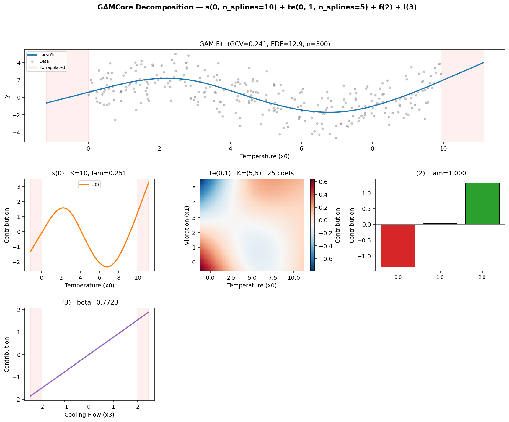
Multi-term GAMCore.plot_decomposition output showing overall fit (top) and isolated partial
dependence panels for s(), te(), f(), and l() terms.