Examples

This chapter collects end-to-end examples demonstrating common use cases.

Runnable notebooks

Three executed notebooks live in examples/. The two backend tutorials walk through the mathematics and workflow of each backend with assertions for every formula:

• examples/gam_tutorial.ipynb: a hands-on tour across both backends, covering underfitting vs. overfitting, EDF interpretation, 2-D tensor interactions, and shape constraints.

• examples/wood_backend_math_tutorial.ipynb: the Wood backend’s mathematics and workflow, covering the basis zoo, S.scale and sum-to-zero absorption, continuous REML/GCV optimisation, Wood (2013) approximate F-tests, and a full engineering case study.

• examples/eilers_backend_math_tutorial.ipynb: the Eilers-Marx backend’s mathematics and workflow, covering De Boor B-splines, difference penalties, the SVD data-augmentation solver, GCV grid search, shape constraints, and the same case study end to end.

Running the notebooks needs the Jupyter stack, which you can install with pip install -e .[notebooks] from the repository root.

Basic regression & residual diagnostics

import numpy as np
from magli import GAMCore

np.random.seed(42)
n = 300
x = np.column_stack([
    np.random.uniform(0, 10, n),
    np.random.uniform(0, 5, n),
])
y = np.sin(x[:, 0]) + 0.3 * x[:, 1] + np.random.normal(0, 0.2, n)

model = GAMCore("s(0, n_splines=12) + l(1)", backend="eilers")
model.fit(x, y)

print("GCV  =", model.statistics_['GCV'])
print("EDF  =", model.statistics_['edof'])
print("AIC  =", model.aic())
print("BIC  =", model.bic())
print("R²   =", model.deviance_explained())

y_hat = model.predict(x)
ci = model.confidence_intervals(x)

fig_decomp, axes_decomp = model.plot_decomposition(x, y)
fig_diag, axes_diag = model.plot_diagnostics(x, y)

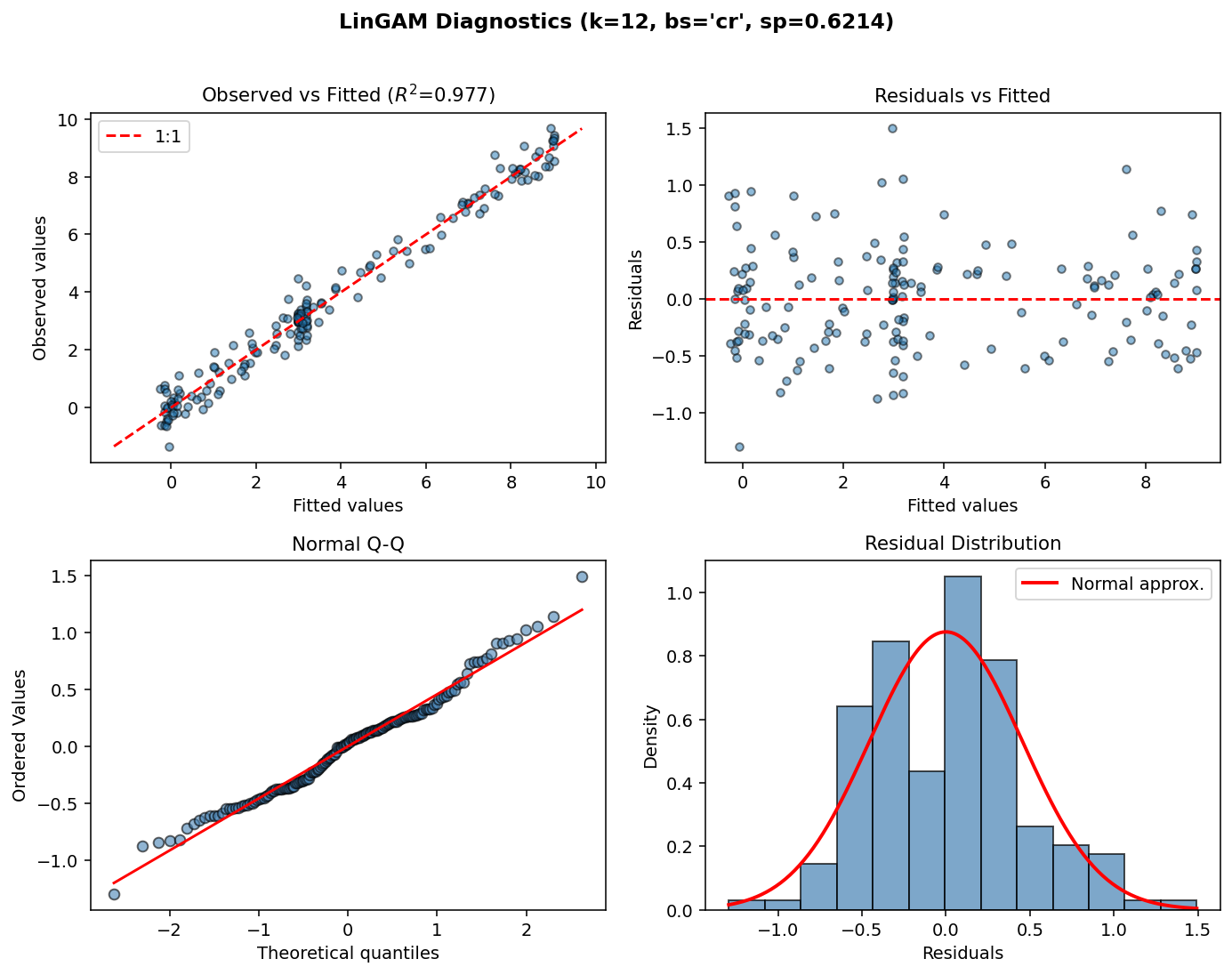
Four diagnostic views produced by model.plot_diagnostics(x, y), showing observed versus fitted values, Residuals vs. Fitted values, Residual Histogram, and Normal Q-Q plot.

Grid search with selective terms

model = GAMCore("s(0) + s(1) + te(0, 1)", backend="eilers")
model.gridsearch(
    x, y,
    lam_grids=[np.logspace(-2, 2, 5)],
    n_splines_grids=[np.arange(5, 13, 2)],
    search_terms=['s'],  # only tune the univariate splines
)

print("Best s(0): K =", model._terms[0].n_splines,
      "lam =", model._terms[0].lam)

Categorical + interaction

np.random.seed(42)
n = 400
x = np.column_stack([
    np.random.uniform(0, 10, n),                    # continuous
    np.random.uniform(0, 5, n),                      # continuous
    np.random.choice([0, 1, 2], n).astype(float),   # categorical
])
y = (
    np.sin(x[:, 0])
    + 0.3 * x[:, 1]
    + np.where(x[:, 2] == 0, -1, np.where(x[:, 2] == 1, 0, 2))
    + np.random.normal(0, 0.3, n)
)

model = GAMCore("s(0) + l(1) + f(2)", backend="eilers")
model.fit(x, y)
model.gridsearch(x, y)

# Partial dependence for each term
pdep_s = model.partial_dependence(0, x)
pdep_l = model.partial_dependence(1, x)
pdep_f = model.partial_dependence(2, x)

Wood backend & summary table

import numpy as np
from magli import GAM

np.random.seed(42)
n = 200
x = np.linspace(0, 1, n)
y = np.sin(2 * np.pi * x) + np.random.normal(0, 0.15, n)

# In Wood backend (the default), lambda (sp) is estimated automatically via REML
model = GAM(k=10, bs="cr", backend="wood")
model.fit(x, y)

# Formatted summary table (Wood 2013)
print(model.summary())
print("Deviance explained:", model.deviance_explained())

Monotonic dose-response

np.random.seed(42)
dose = np.random.uniform(0, 10, 150)
response = 5 * (1 - np.exp(-0.4 * dose)) + np.random.normal(0, 0.3, 150)

model = GAM(n_splines=12, constraint='mono_inc', backend="eilers")
model.fit(dose, response)

# Grid search respects the monotonic constraint
model.gridsearch(dose, response)

fig, axes = model.plot_decomposition(dose, response)

Periodic seasonal pattern

np.random.seed(42)
hour = np.random.uniform(0, 24, 300)
temp = (
    20
    + 8 * np.sin(2 * np.pi * hour / 24)
    + 3 * np.random.normal(0, 1, 300)
)

# Periodic constraint encloses the daily cycle
model = GAM(n_splines=12, constraint='periodic', backend="eilers")
model.fit(hour, temp)

# Predict across a full day
hour_grid = np.linspace(0, 24, 200)
temp_hat = model.predict(hour_grid)

# 6 AM and 6 PM should have the same prediction as 30 h and 42 h
assert np.isclose(model.predict([6]), model.predict([30]), atol=1e-3)

Observation weights for outlier resistance

import numpy as np
from magli import GAM

np.random.seed(42)
x = np.linspace(0, 10, 150)
y = np.sin(x) + np.random.normal(0, 0.18, len(x))
y[[20, 55, 95, 130]] += np.array([3.2, -3.0, 3.4, -2.8])  # sensor spikes

# Initial fit and MAD-scaled Huber weights
m0 = GAM(k=14, bs="cr", backend="wood").fit(x, y)
resid = y - m0.predict(x)
mad_sigma = 1.4826 * np.median(np.abs(resid - np.median(resid)))
u = np.abs(resid) / (mad_sigma + 1e-12)
weights = np.where(u <= 1.345, 1.0, 1.345 / u)

# Refit with observation weights (supported in both backends)
m_weighted = GAM(k=14, bs="cr", backend="wood").fit(x, y, weights=weights)

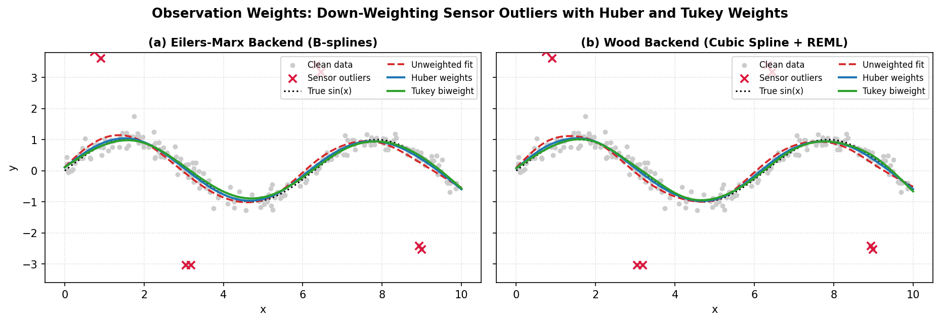
Down-weighting sensor spikes via weights=... prevents outliers from pulling the smooth curve in both the Eilers-Marx and Wood backends.

2-D tensor interaction

np.random.seed(42)
n = 500
x = np.column_stack([
    np.random.uniform(0, 10, n),
    np.random.uniform(0, 5, n),
])
y = (
    np.sin(x[:, 0]) * np.cos(x[:, 1])
    + 0.5 * x[:, 0]
    + np.random.normal(0, 0.3, n)
)

model = GAMCore("s(0) + s(1) + te(0, 1, n_splines=6)", backend="eilers")
model.fit(x, y)
model.gridsearch(x, y)

# te(0,1) captures the interaction that s(0)+s(1) cannot
pdep_te = model.partial_dependence(2, x)

fig, axes = model.plot_decomposition(x, y)