Part II — The Eilers & Marx Backend

Tip

A runnable companion to this chapter ships with the repository: examples/eilers_backend_math_tutorial.ipynb. It follows the same order, rebuilds the Cox-de Boor recursion by hand, checks the difference penalty and the singular normal equations (X^T X + P has a one-dimensional null space that the solver’s augmentation ridge repairs), and ends with a pass/fail audit.

How the Eilers-Marx backend thinks

The Eilers-Marx backend (backend='eilers') is the minimalist design, relying on one basis family, one solver, one criterion, chosen well. Every smooth term is a uniform cubic B-spline; smoothness is charged by a difference penalty; the one free knob, the smoothing parameter \(\lambda\), is chosen by evaluating a discrete grid of candidates and keeping the one with the best Generalised Cross Validation (GCV) score.

The whole pipeline is:

\[\text{formula} \;\to\; \underbrace{B\text{-spline bases } X}_{\S 1} \;\to\; \underbrace{\text{penalty } P}_{\S 2} \;\to\; \underbrace{\text{solve } (X^\top X + P)\hat\beta = X^\top y}_{\S 3--4} \;\to\; \underbrace{\text{score with GCV, pick best } (K, \lambda)}_{\S 5--6}.\]

Each step is a section below. The design bets on three ideas:

1. Uniform B-splines are good enough. A cubic B-spline with 10-20 basis functions can approximate almost any smooth engineering relationship; the exact knot placement rarely matters at that resolution.

2. Grid search is honest. Instead of optimising \(\lambda\) continuously (which requires derivatives of criteria that may have flat or multiple minima), evaluate a finite, user-visible grid and pick the winner. Slow in theory, fast in practice once you precompute cleverly (grid search).

3. SVD is the safest solver. Never form \(X^\top X\) explicitly; work with a square-root of the penalised system instead (SVD solver).

Identifiability in this backend is implicit, meaning the intercept column is unpenalised and absorbs the overall level, and each penalty leaves its own null space (constant and linear trends for the default penalty) uncharged, so the decomposition into intercept + smooths is well defined in practice. There is no explicit centering constraint, a deliberate simplification we compare against Wood’s approach later.

B-Spline Bases and Local Building Blocks

If we want \(f(x)\) to be a smooth, flexible curve, we need a way to represent it mathematically.

Why not just use a high-degree polynomial? A degree-20 polynomial can wiggle a lot, but when you fit it to data every point in one corner of the plot affects the curve everywhere. You get wild oscillations (Runge’s phenomenon). Polynomials are globally coupled, so changing one coefficient moves everything changes.

The central principle of B-splines is to build the curve from localised building blocks. Each block (basis function) is nonzero only in a small region. Adjusting a block only changes the curve in its neighbourhood, not across the whole domain. This is called compact support.

Think of LEGO bricks. A long, curved wall isn’t built from one flexible piece; instead, it is built from many small, rigid bricks each responsible for a tiny segment. The bricks overlap slightly at the edges for smoothness. B-spline basis functions are the mathematical equivalent. Each one is a smooth “bump” that covers a few neighbouring data points. When you stack them with different heights (coefficients \(\beta_j\)), you get any smooth shape you want:

\[f(x) = \sum_{j=1}^K \beta_j \, B_j(x).\]

Each \(B_j(x)\) is one basis function; \(\beta_j\) is how tall you make it; \(K\) is how many bricks you use (n_splines or k in the API).

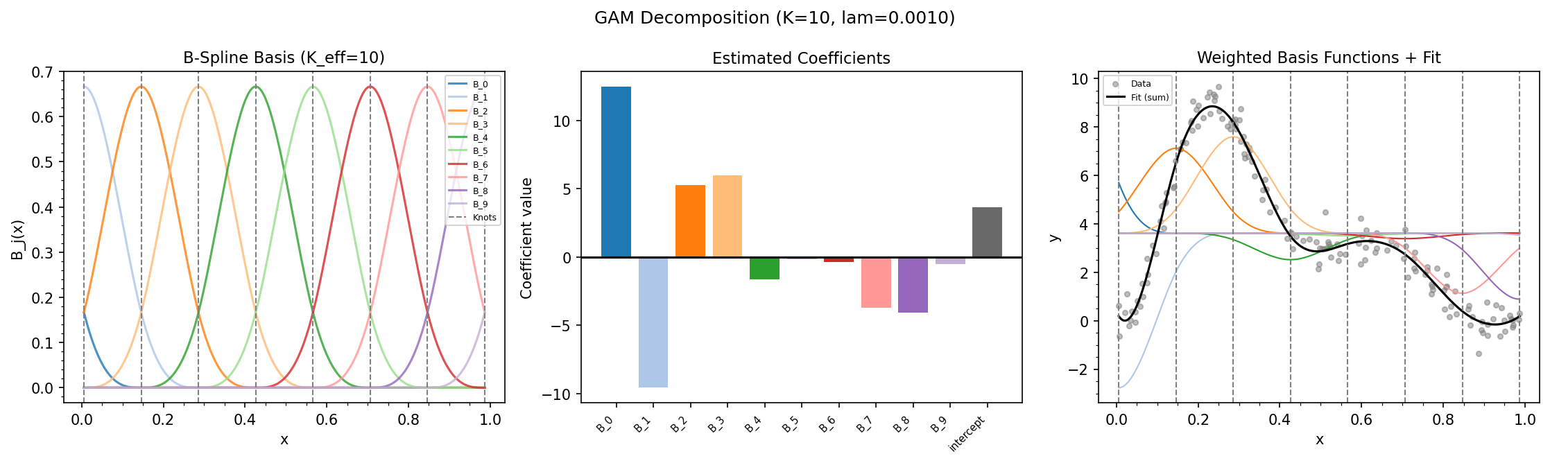
Single-term LinGAM.plot_decomposition (Eilers-Marx backend), showing (left) uniform cubic B-spline basis bumps \(B_j(x)\) and interior knots, (middle) estimated coefficients \(\hat\beta_j\) and intercept, (right) scaled basis functions \(\hat\beta_j B_j(x) + \hat\beta_0\) summing to the fitted curve.

The De Boor recursion. A B-spline of polynomial degree \(k\) (order \(k+1\), spline_order=k in the API) is built recursively. Given data \(x \in [x_{\min}, x_{\max}]\), we map to \([0, 1]\):

\[z = \frac{x - x_{\min}}{x_{\max} - x_{\min}}.\]

Uniform interior knots (\(1 + K - k\) points) divide \([0, 1]\) into \(K - k\) segments:

\[\tau_0 = 0, \; \tau_1, \dots, \tau_{K-k} = 1.\]

The augmented knot sequence extends \(k\) knots beyond each boundary to handle the edges.

Start with order-1 (piecewise constant) bases:

\[B_{i,1}(z) = \mathbf{1}_{[\tau_i, \tau_{i+1})}(z).\]

Then recursively blend for orders \(m = 2, \dots, k+1\):

\[B_{i,m}(z) = \frac{z - \tau_i}{\tau_{i+m-1} - \tau_i} \, B_{i,m-1}(z) + \frac{\tau_{i+m} - z}{\tau_{i+m} - \tau_{i+1}} \, B_{i+1,m-1}(z).\]

Each blend raises the order by one and shrinks the basis count by one, so \(K\) functions of order \(k+1\) come out at the end. The result is an \(n \times K\) design matrix \(B\). Each row sums to 1 (the bricks tile the space) and each column has compact support (localised bumps).

Why cubic? magli defaults to spline_order=3, which the recursion above turns into basis functions of order \(k+1 = 4\), producing cubic polynomials, degree 3. Cubic is the lowest degree that gives continuous second derivatives, so the curve looks smooth to the human eye. Lower orders look jagged; higher orders increase computation without visible benefit.

Linear extrapolation. Outside \([0,1]\), B-splines can oscillate or collapse to zero, which is not useful for prediction beyond the training range. magli replaces the B-spline values with a linear extension using the boundary derivative:

\[f(z) \approx f(0) + f'(0) \, z \quad (z < 0), \qquad f(z) \approx f(1) + f'(1) \, (z-1) \quad (z > 1).\]

The derivative \(f'(0)\) is computed analytically from the order-\(k\) bases saved during the last step of the recursion, using the standard B-spline derivative formula \(B'_{i,k+1} = k \bigl( B_{i,k}/\Delta\tau - B_{i+1,k}/\Delta\tau \bigr)\).

Periodic basis. When constraint='periodic', the domain wraps around by evaluating the input modulo 1 and folding the last \(k\) columns into the first \(k\), preserving the partition of unity \(\sum_j B_j(x) = 1\), enforcing \(f(0) = f(1)\), and reducing the coefficient count from \(K\) to \(K_{\text{eff}} = K - k\).

Penalties and the Cost of Flexibility

Suppose we give the model \(K = 30\) basis functions. It could fit the data almost perfectly, including every random noise wiggle. When we then predict on new data, the model falls apart. This is overfitting.

The solution is to penalise complexity. We don’t forbid wiggles; we charge a tax for them. The model can still wiggle, but only if doing so improves the fit enough to be worth the tax.

The penalised least-squares objective is:

\[\underbrace{\|\mathbf{y} - X\boldsymbol{\beta}\|^2}_{\text{fit to data}} \;+\; \underbrace{\boldsymbol{\beta}^\top P \boldsymbol{\beta}}_{\text{complexity penalty}}.\]

The first term rewards fitting the training data closely. The second term punishes certain patterns in the coefficients. The smoothing parameter \(\lambda\) (lam in the API) controls the tax rate:

• Zero penalty (\(\lambda = 0\)): the curve can be as wiggly as the basis allows (equivalent to unpenalised regression).

• Infinite penalty (\(\lambda \to \infty\)): the curve is forced to be as smooth as possible (a straight line for second-difference penalties).

• Balanced penalty (\(0 < \lambda < \infty\)): magli uses grid search to find the \(\lambda\) that minimises GCV.

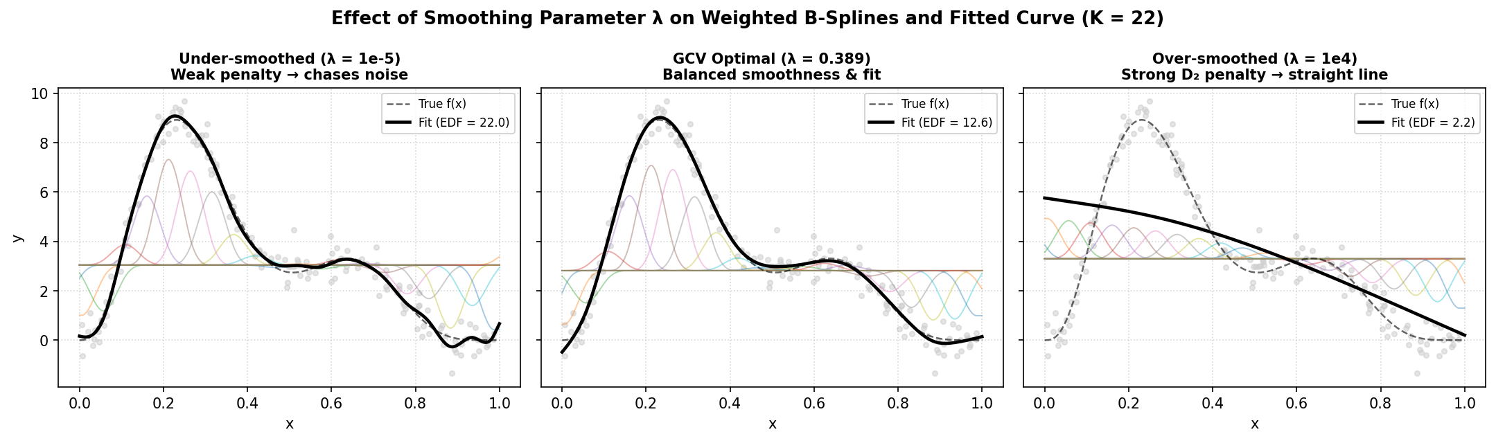
How \(\lambda\) shapes the fit (\(K = 22\)), showing (left) weak penalty (\(\lambda = 10^{-5}\)) lets adjacent B-splines oscillate to chase noise; (middle) GCV-optimal \(\lambda\) balances smoothness and fidelity; (right) strong penalty (\(\lambda = 10^4\)) forces the second differences to zero, collapsing the curve onto its linear null space (\(\text{EDF} \approx 2\)).

What each penalty does to the curve:

Second-difference penalty (default). Penalises the curvature (second derivative) of \(f(x)\). A straight line has zero curvature, so it costs nothing. Wiggles cost a lot, producing the visually smooth curves we expect.

\[\begin{split}D_2 = \begin{pmatrix} 1 & -2 & 1 & & \\ & 1 & -2 & 1 & \\ & & \ddots & \ddots & \ddots \end{pmatrix}_{(K-2) \times K}, \qquad P = \lambda \, D_2^\top D_2.\end{split}\]

Active-set directional shape penalties (mono_inc, mono_dec, convex, concave). In addition to the smoothness penalty \(\lambda D_2^\top D_2\), shape-constrained terms add pyGAM’s iterative active-set penalty \(C(\boldsymbol{\beta}) = \lambda_{\text{con}} D_m^\top \operatorname{diag}(\mathbf{v}(\boldsymbol{\beta})) D_m + \lambda_{L2} I\) with \(\lambda_{\text{con}} = 10^9\) and \(\lambda_{L2} = 10^{-3}\), where \(\mathbf{v}(\boldsymbol{\beta})\) selects violated first differences (\(m=1\) for monotonicity) or second differences (\(m=2\) for convexity/concavity).

Circular second-difference (periodicity). The second-difference operator wraps around, connecting the last coefficient back to the first, which is the mathematical equivalent of gluing the two ends of the curve together.

Ridge penalty. For factor terms (and linear terms, if penalised), \(P = \lambda I_K\). This is a “shrink-toward-zero” penalty that pulls all coefficients toward zero by the same amount. (Linear l() terms default to \(\lambda = 0\), remaining unpenalised.)

The role of \(\boldsymbol{\lambda}\) cannot be overstated. \(\lambda\) determines how much information the model extracts from the data vs. how much it imposes from the smoothness prior. Too small → overfitting (the model chases noise). Too large → underfitting (the model misses real patterns). Grid search finds the Goldilocks value automatically.

The SVD data-augmentation solver

Once we have the design matrix \(X\) and the penalty \(P\), we need to find the coefficients \(\hat{\boldsymbol{\beta}}\) that minimise the penalised objective.

The naive approach forms the normal equations:

\[(X^\top X + P)\hat{\boldsymbol{\beta}} = X^\top \mathbf{y}.\]

This is mathematically correct but numerically dangerous. Forming \(X^\top X\) squares the condition number: if \(X\) has a condition number of \(10^4\), then \(X^\top X\) has \(10^8\). On a computer with 16-digit precision, this leaves very little room for error.

The data-augmentation trick treats the penalty as “fake data”:

\[\begin{split}\begin{pmatrix} X \\ E \end{pmatrix} \boldsymbol{\beta} \approx \begin{pmatrix} \mathbf{y} \\ \mathbf{0} \end{pmatrix},\end{split}\]

where \(E\) satisfies \(E^\top E = P + \sqrt{\varepsilon}\, I\) (a tiny ridge \(\sqrt{\varepsilon}\) with machine epsilon \(\varepsilon\) ensures positive definiteness even when \(\lambda = 0\); in solve_pirls \(E\) is the transposed Cholesky factor of \(P + \sqrt{\varepsilon}\, I\)). The top block says “fit the actual data.” The bottom block says “keep the coefficients small in the penalised directions.”

Solving this augmented system is equivalent to the penalised normal equations, but never forms \(X^\top X\). Instead, magli uses:

1. QR decomposition of \(X = QR\). \(R\) is small (\(m \times m\), where \(m = \sum K_j + 1\)), so subsequent operations are cheap even when \(n\) is huge.

2. SVD of the stacked matrix \([R; E] = U \Sigma V^\top\). The singular value decomposition is the most numerically stable way to factor a matrix; it exposes the “directions” in which the data has information and the directions it doesn’t.

3. Solution operator \(B_{\text{solve}} = V \Sigma^{-1} U_1^\top Q^\top\) so that \(\hat{\boldsymbol{\beta}} = B_{\text{solve}} \mathbf{y}\). This is saved and reused for covariance, EDF, and confidence intervals with no re-solving needed. (\(U_1\) is the top \(m \times m\) block of \(U\), the part corresponding to the data block \(R\).)

The SVD approach is especially important when \(\lambda\) is very small (the near-unpenalised case) or very large (near-zero coefficients), where the normal equations become ill-conditioned. By working with the square-root of \(X^\top X + P\) rather than the matrix itself, the SVD solver stays accurate across the entire range of \(\lambda\).

Effective Degrees of Freedom (EDF)

In ordinary linear regression with \(p\) predictors, the model uses exactly \(p\) degrees of freedom, one per coefficient. You can think of each degree of freedom as the model’s ability to “move” in one independent direction to fit the data.

Penalised splines blur this picture. The model has \(K\) coefficients (basis functions), but the penalty restricts how freely each one can move. A heavily penalised coefficient is “shrunken” toward its neighbours, costing an entire degree of freedom to include, but the penalty means you only use a fraction of it.

The EDF measures how many independent directions the fitted model actually explores. It is always between 0 and \(K\), and usually much closer to the number of “real features” in the data.

Mathematically, the EDF is the trace of the influence (hat) matrix:

\[\text{EDF} = \operatorname{tr}(H), \qquad H = X (X^\top X + P)^{-1} X^\top.\]

Using the SVD augmentation from the solver, this simplifies to:

\[\text{EDF} = \sum_{i} \sigma_i(U_1)^2 = \|U_1\|_F^2,\]

where \(U_1\) is the data block of the SVD’s left singular vectors. To understand why this equality holds, observe that with \(X = QR\) and \([R;E] = U\Sigma V^\top\), the hat matrix factors as \(H = Q U_1 U_1^\top Q^\top\), so its trace is \(\operatorname{tr}(U_1^\top Q^\top Q U_1) = \|U_1\|_F^2\). This is computed in a single NumPy call with no matrix inversion.

In practice, the estimated EDF offers immediate insight into what your model learned:

• An EDF near 2 indicates that the term has essentially collapsed to a linear slope.

• An EDF close to the basis dimension \(K\) shows that the penalty is very weak and the term is using almost its full parameter capacity.

• An EDF substantially lower than \(K\) with a strong fit confirms that the penalty is working as intended, capturing a smooth trend with just a few effective parameters.

• An EDF growing while the GCV score stays flat warns of overfitting, where additional wiggles chase noise without improving predictive accuracy.

Per-direction EDF is stored in statistics_['edof_per_coef']:

\[\text{EDF}_j = \sum_i U_{1,ji}^2 = (U_1 U_1^\top)_{jj}.\]

In the Eilers-Marx SVD solver, the rows of \(U_1\) correspond to the \(m\) QR-orthogonalised directions of \(R\) (\(Q^\top H Q = U_1 U_1^\top\)), whereas the Wood backend reports the diagonal of the coefficient influence matrix \(F = (X^\top X + S_\lambda)^{-1} X^\top X\) directly in the spline basis coordinates; both sum to the exact same total \(\text{EDF} = \operatorname{tr}(H)\).

Generalised Cross Validation (GCV)

The problem. How do we know if our model is good? We could hold out some data, fit on the rest, and check how well it predicts the held-out points. But we’d have to do this many times (cross-validation), which is slow, especially during grid search where we evaluate thousands of models.

The clever solution. Leave-one-out cross-validation (LOOCV) fits the model \(n\) times, each time dropping one data point and predicting it. This is \(O(n)\) fits, prohibitive for anything but tiny datasets.

GCV is a closed-form approximation of LOOCV that requires only one fit. The formula:

\[\text{GCV} = \frac{n \cdot \text{RSS}} {(n - \gamma \cdot \text{EDF})^2}.\]

Let’s unpack each piece:

• Sample size \(n\): a larger dataset gives a more stable estimate.

• Residual sum of squares \(\text{RSS} = \sum_i (y_i - \hat y_i)^2\): measures how far the predictions are from the actual values (lower is better).

• \(\text{EDF}\) represents effective degrees of freedom, measuring the model’s complexity. More EDF means the model can “chase” data points more aggressively.

• \(\gamma\) is the GCV penalty multiplier (default 1.4 in the Eilers-Marx backend). Setting \(\gamma > 1\) makes the criterion slightly conservative, preferring simpler models in analogy to AIC’s penalty term.

The denominator \((n - \gamma \cdot \text{EDF})^2\) is the key. When EDF is small (simple model), the denominator is large → GCV is small → good. When EDF grows, the denominator shrinks → GCV explodes → bad, unless the extra complexity reduces RSS enough to compensate.

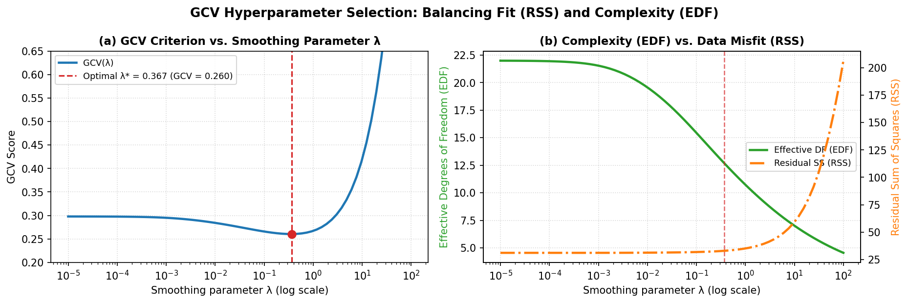
(a) The GCV score attains a minimum at \(\lambda^*\) where the reduction in RSS no longer justifies the complexity penalty \((n - \gamma\cdot\text{EDF})^{-2}\). (b) As \(\lambda\) increases, EDF decreases smoothly toward the null-space dimension while RSS increases monotonically.

Why GCV and not plain CV? GCV is asymptotically equivalent to LOOCV but computes in \(O(1)\) extra time after a single fit. It’s the reason magli’s grid search can evaluate thousands of hyperparameter combinations in seconds rather than minutes.

Interpreting GCV values:

• GCV is in squared units of \(y\). Comparing GCV between models on the same dataset tells you which is better; comparing across datasets does not.

• A GCV that drops dramatically when you add a term means the term is useful.

• A GCV that stays flat or increases when you add a term means the term is unnecessary noise.

• The absolute value matters less than the relative value across models.

Putting the Penalized Fit Together

Let’s trace what happens when you call model.fit(x, y) with the Eilers-Marx backend:

1. Parse the formula. "s(0) + te(1,2) + f(3)" becomes a list of term objects, each knowing its feature column(s), basis count, and penalty type.

2. Build design matrices. Each term constructs its B-spline basis (or one-hot encoding for factors, or just a column for linear terms). These are stacked side-by-side, plus an intercept column of ones, to form the full design matrix \(X\) with dimensions \(n \times m\).

3. Build the penalty. Each term’s penalty matrix is computed and assembled into a block-diagonal \(P\) with dimensions \(m \times m\). The intercept block is kept at zero because we never penalize the overall baseline level.

4. Solve. The SVD data-augmentation solver finds \(\hat{\boldsymbol{\beta}}\) and stores the solution operator \(B_{\text{solve}}\) for later use.

5. Compute diagnostics. RSS, EDF, GCV, scale estimate, covariance matrix, standard errors, all accessible via model.statistics_.

Why the intercept is special. If we penalised the intercept, the model would be forced toward \(y = 0\), which is almost never what we want. The intercept absorbs the overall level, letting the penalised terms focus on shape. This is why fit_intercept=True is the default and why the intercept block in \(P\) is zero.

A note on identifiability. The default second-difference penalty does not charge constant or linear trends (they lie in \(D_2\)’s null space). Together with the unpenalised intercept, this pins down the decomposition, so the intercept owns the level, and each smooth owns only its bending. The Eilers-Marx backend relies on this implicit mechanism. The Wood backend, as we’ll see, makes the centering explicit with a sum-to-zero constraint (same goal, different route).

Tensor-product interactions

An additive model with only univariate terms cannot capture relationships where the effect of one predictor depends on the value of another. For example, high temperature might be especially damaging at high vibration, representing a synergistic interaction.

The tensor product te(f1, f2, ..., fd) models this by building a multi-dimensional smooth surface. The design matrix is the column-wise Kronecker product of marginal B-spline bases:

\[B_{\text{tensor}} = B_1 \odot B_2 \odot \dots \odot B_d.\]

If \(B_1\) is \(n \times K_1\) and \(B_2\) is \(n \times K_2\), then \(B_{\text{tensor}}\) is \(n \times (K_1 K_2)\). This grows quickly. For example, a 2-D tensor with \(K_1 = K_2 = 6\) creates 36 columns; with \(K_1 = K_2 = 10\) it’s 100 columns. This is why tensor terms use smaller default \(K\) values (4-8) than univariate splines (5-25).

The penalty is assembled as a Kronecker sum, giving each dimension its own smoothing parameter:

\[P_{\text{tensor}} = \sum_{d=1}^D \lambda_d \, \bigl( I_{K_1} \otimes \dots \otimes P_d \otimes \dots \otimes I_{K_D} \bigr).\]

This means smoothness is enforced independently in each direction. A surface can be smooth in temperature but wiggly in vibration, or vice versa. (Pass a list to lam= to give each dimension its own \(\lambda_d\); a scalar is broadcast to all dimensions.)

When to use a tensor vs. separate s() terms. If the interaction exists, a model with only s(temperature) + s(vibration) will show patterned residuals, as the error at high temperature and high vibration will be systematically wrong. Adding te(temperature, vibration) captures this extra structure. You can verify this in the decomposition plot; if the te() heatmap shows a strong diagonal pattern, the interaction is real.

Confidence and prediction intervals

A point prediction says “the model thinks blade life is 42.3 cycles.” An interval says “the model thinks blade life is between 40.1 and 44.5 cycles, with 95% confidence.” Intervals quantify uncertainty.

Confidence intervals quantify uncertainty about the true average response at a given point, reflecting variability in the coefficient estimates. They are narrow where data is abundant and wider where data is sparse.

Prediction intervals assess where a single new observation would likely fall, combining coefficient uncertainty with residual variability \(\hat\sigma^2\). A prediction interval is always wider than a confidence interval at the same point, because individual observations are inherently noisier than population averages.

The formulas:

\[\text{Var}(\hat y(\mathbf{x}^*)) = \mathbf{x}^{*\top} \, \text{Cov}(\hat{\boldsymbol{\beta}}) \, \mathbf{x}^*,\]

\[\text{Cov}(\hat{\boldsymbol{\beta}}) = B_{\text{solve}} B_{\text{solve}}^\top \, \hat\sigma^2, \qquad \hat\sigma^2 = \frac{\text{RSS}}{n - \text{EDF}}.\]

Confidence intervals:

\[\hat y(\mathbf{x}^*) \pm t_{\alpha/2, \, n-\text{EDF}} \, \sqrt{\text{Var}(\hat y(\mathbf{x}^*))}.\]

Prediction intervals:

\[\hat y(\mathbf{x}^*) \pm t_{\alpha/2, \, n-\text{EDF}} \, \sqrt{\text{Var}(\hat y(\mathbf{x}^*)) + \hat\sigma^2}.\]

We use the t-distribution (not the normal) because \(\sigma\) is estimated from the data. Degrees of freedom are \(n - \text{EDF}\) because the penalty has already “used up” EDF worth of information.

This covariance is the frequentist one, treating \(\lambda\) as fixed and propagates only the sampling variability of \(\hat{\boldsymbol{\beta}}\). The Wood backend additionally computes a Bayesian covariance (treating the penalty as a prior); the difference is explained in Part III.

How Fast Grid Search Works

Grid search evaluates every combination of \(K\) (n_splines) and \(\lambda\) (lam) candidates. A naïve implementation would rebuild \(X\) and solve from scratch for each combination, which is prohibitively slow.

magli’s fast path splits the work into two phases:

Phase 1 — Precompute per \(\boldsymbol{K}\) (threaded). For each candidate basis count \(K\):

1. Build \(X_K\) and compute \(X_K = Q_K R_K\) (QR).

2. Cache \(R_K^\top R_K\) and \(R_K^\top Q_K^\top \mathbf{y}\). These are independent of \(\lambda\).

3. Precompute the unscaled penalty basis \(S = D^\top D\) at \(\lambda = 1\).

All \(K\)-configurations are processed in parallel when n_jobs != 1 (ThreadPoolExecutor; NumPy releases the GIL during QR decomposition, so CPU-bound linear algebra genuinely runs on multiple cores). With the default n_jobs=1 everything runs serially.

Phase 2 — Evaluate per \(\boldsymbol{(K, \lambda)}\) (threaded). For each combination:

1. Assemble the penalty matrix \(P = \lambda S\).

2. Form \(B = R_K^\top R_K + P\).

3. Cholesky solve for \(\hat{\boldsymbol{\beta}}\) and EDF.

4. Compute RSS and GCV.

Cholesky costs \(O(m^3/3)\) vs. \(O(m^3)\) for SVD, and it’s numerically safe because \(R_K^\top R_K + P\) is positive definite (the penalty adds ridge stabilisation). Both the K-precomputation and the per-K evaluation loop use the same n_jobs-gated threading.

Why this matters. For a model with \(m = 20\) coefficients, \(n = 500\) observations, and a grid of \(8 \times 8 = 64\) combinations, whereas a direct unoptimized sweep takes ~64 SVDs of \(500 \times 20\) matrices. The fast path does ~8 QR decompositions (one per unique \(K\)) and ~64 Cholesky solves (one per \((K, \lambda)\) pair), which is roughly 10× faster. The gap widens with larger \(n\).

Each smooth term (and each tensor dimension) owns its own \(\lambda\) slot in the grid, so the search optimises a vector of smoothing parameters jointly. A scalar lam= grid is broadcast to every slot when you want the classic “one \(\lambda\) for the whole model” behaviour.

Observation weights

Both backends accept a 1-D vector of non-negative observation weights \(\mathbf{w} = (w_1, \dots, w_n)\) in fit(x, y, weights=w) and gridsearch(x, y, weights=w) to minimise the weighted penalised least-squares objective:

\[\sum_{i=1}^n w_i (y_i - \mathbf{x}_i^\top \boldsymbol{\beta})^2 + \boldsymbol{\beta}^\top P \boldsymbol{\beta} = \|\mathbf{W}^{1/2}(\mathbf{y} - X\boldsymbol{\beta})\|^2 + \boldsymbol{\beta}^\top P \boldsymbol{\beta}.\]

Numerically, magli pre-multiplies each row of \(X\) and each element of \(\mathbf{y}\) by \(\sqrt{w_i}\) before calling the standard solver. This supports:

• Precision / inverse-variance weighting (\(w_i = 1 / \sigma_i^2\)) for heteroskedastic measurements.

• Frequency / replicate weights for grouped observations.

• Outlier down-weighting by assigning small weights (e.g. single-pass MAD-scaled Huber or Tukey biweight weights) to flagged sensor glitches.

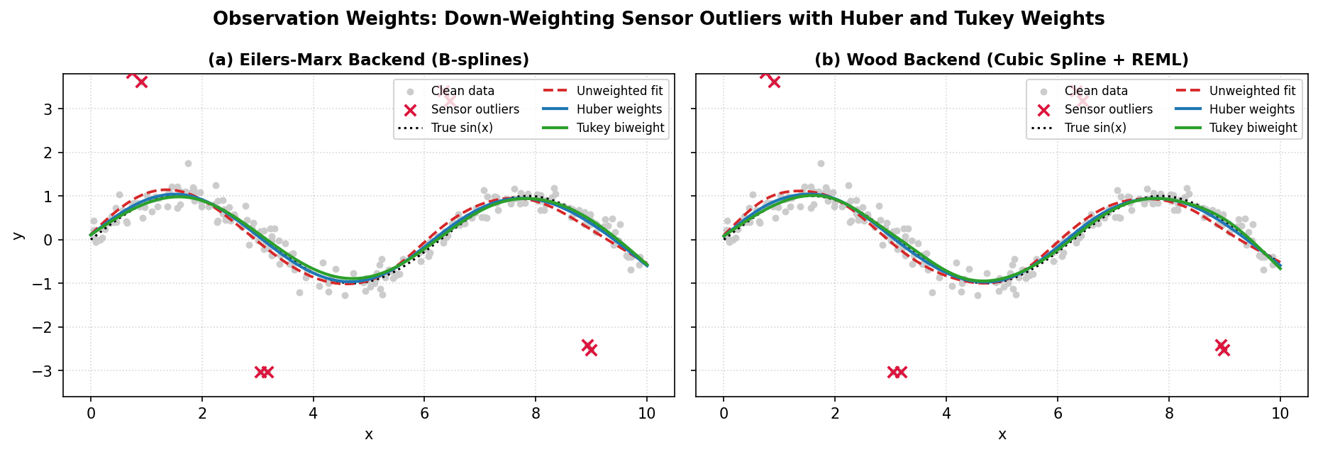
Passing MAD-scaled Huber or Tukey biweight observation weights to fit() prevents gross sensor outliers (red crosses) from distorting the smooth curve in both the Eilers-Marx and Wood backends.