Part III — The Wood Backend¶

Tip

A runnable companion to this chapter ships with the repository: examples/wood_backend_math_tutorial.ipynb. It follows the same order, recomputes every identity below numerically (Green’s function, S = D^T B^{-1} D, the sum-to-zero absorption, the REML criterion and its analytic gradient), and ends with a pass/fail audit.

How the Wood backend thinks¶

The Wood backend (backend='wood') is a pure Python implementation of Simon Wood’s GAM framework (Wood 2006, 2011, 2017). Where the Eilers-Marx backend bets on one basis and a grid search, Wood bets on richness and automatic inference:

A zoo of bases. Nine basis codes ('tp', 'ts', 'cr', 'cs', 'cc', 'ps', 'cp', 'bs', 're') with different knot placements, different penalties, and different shrinkage behaviour. Each solves the smoothness problem a slightly different way.
One smoothing parameter per penalty, estimated. Instead of sweeping a grid, the backend treats $\lambda$ as a free parameter and optimises a model-selection criterion, using Restricted Maximum Likelihood (REML) by default, GCV as an option, in log-$\lambda$ space with standard optimisers.
Explicit identifiability. Every smooth is centred by absorbing a sum-to-zero constraint into the basis itself, and every penalty is rescaled to a common scale (S.scale), so the $\lambda$ values are comparable across terms.
Full inferential machinery. Bayesian and frequentist covariances, per-term approximate F-tests with p-values (Wood 2013), AIC/BIC, deviance explained.

The pipeline is:

\[\text{formula} \;\to\; \underbrace{\text{basis + penalty per term}}_{\S 1} \;\to\; \underbrace{\text{rescale, centre}}_{\S 2} \;\to\; \underbrace{\text{optimise } \lambda \text{ by REML/GCV}}_{\S 3} \;\to\; \underbrace{\text{inference}}_{\S 4}.\]

Sections 1-4 below follow that order.

The basis zoo¶

All of the Wood bases share one objective, representing a smooth $f(x)$ as a linear combination of basis functions with an attached wiggliness penalty $\boldsymbol{\beta}^\top S \boldsymbol{\beta}$. Four of the families (tp, cr, cc, bs) penalise an exact derivative integral $\int (f^{(m_2)}(x))^2\,dx$; the P-spline families (ps, cp) penalise discrete differences of coefficients; the random effect family (re) penalises the coefficients directly. Here’s the map:

Code	Family	Basis functions	Penalises	Null space
`tp`	Thin plate regression spline	$k$ leading eigenfunctions of the curvature kernel	$\int f''^2 dx$	constants + linear (dim 2)
`ts`	Thin plate, shrinkage	same as `tp`	curvature + small charge on the null space	none (can shrink to zero)
`cr`	Cubic regression spline	natural cubics, knots at sample quantiles	$\int f''^2 dx$	linear functions (dim 2)
`cs`	Cubic, shrinkage	same as `cr`	curvature + small charge on the null space	none (can shrink to zero)
`cc`	Cyclic cubic	periodic natural cubics	$\int f''^2 dx$ on the circle	constants (dim 1)
`ps`	P-spline (Eilers & Marx)	cubic B-splines, equally spaced knots	$m$-th order differences of coefficients	polynomials of degree $< m$
`cp`	Cyclic P-spline	cubic B-splines on wrapped knots	wrapped $m$-th order differences of coefficients	constants (dim 1)
`bs`	B-spline	degree-$m_1$ B-splines (default cubic), equally spaced knots	exact integral $\int \bigl(f^{(m_2)}(x)\bigr)^2 dx$	polynomials of degree $< m_2$
`re`	Random effect	one column per factor level	$\sum \beta_j^2$ (ridge)	none (all levels shrunken)

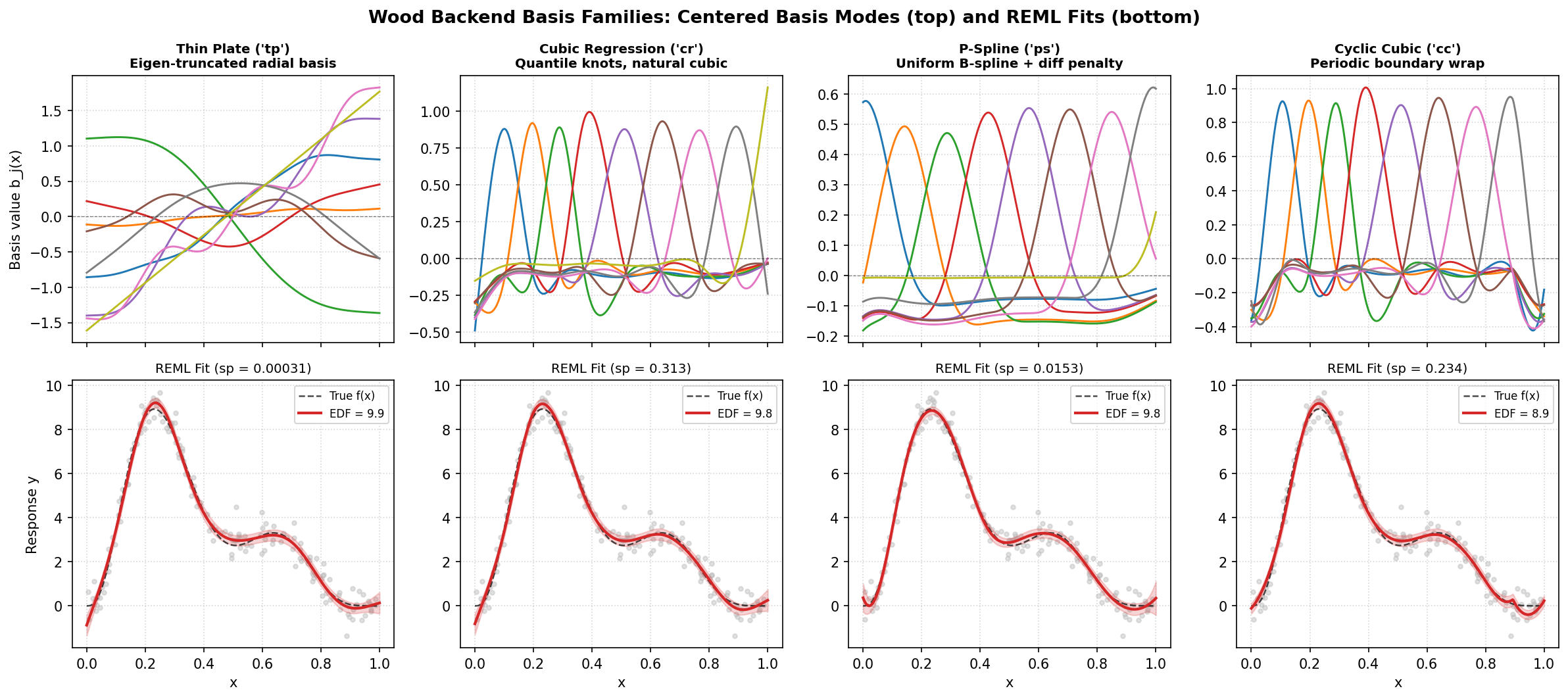
Comparison of four Wood basis families (tp, cr, ps, cc) showing centered basis modes and REML fits — Four representative families from the Wood basis zoo ($k = 10$). The top row shows centred basis modes after absorbing the sum-to-zero constraint (notice how `tp` orders modes from global low-frequency to local high-frequency, whereas `cr` and `ps` localise bumps around knots), while the bottom row shows REML-fitted smooths and 95% Bayesian credible bands on the same noisy signal, with `cc` enforcing periodic wrap-around at the boundaries.¶

The table’s “null space” column matters more than it looks, because those are the function shapes that cost nothing to include. A penalty with a null space leaves the corresponding pattern unpenalised and lets the intercept (or the model’s other terms) absorb it.

Thin plate regression splines (`tp`, `ts`)¶

The default in the Wood backend, and the most mathematically interesting family. It starts from a continuous problem, not a knot placement.

The continuous problem. Among all functions with two derivatives, find the $f$ minimising

\[\sum_{i=1}^n \bigl( y_i - f(x_i) \bigr)^2 + \lambda \int f''(x)^2 \, dx.\]

The first term is ordinary least squares; the second charges the total squared curvature. It turns out (the representer theorem for splines) that the minimiser has the form

\[f(x) = \sum_{i=1}^n \delta_i \, \eta(|x - x_i|) + \alpha_0 + \alpha_1 x, \qquad \eta(r) = \frac{|r|^3}{12},\]

subject to $\sum_i \delta_i = \sum_i \delta_i x_i = 0$ (the $T^\top\delta = 0$ constraint). The $n$ “radial” basis functions sit one on each data point; the two polynomial terms form the null space, meaning they have zero curvature and the penalty never touches them.

Why $\boldsymbol{\eta(r) = |r|^3/12}$ ? It is the Green’s function of the fourth-derivative operator:

\[\frac{d^4}{dr^4}\left(\frac{|r|^3}{12}\right) = \delta(r),\]

where $\delta$ is the Dirac delta. As a consequence, for any function of this form, the curvature integral collapses to a quadratic form in the coefficients,

\[\int f''(x)^2 \, dx \;=\; \boldsymbol{\delta}^\top E \boldsymbol{\delta}, \qquad E_{ij} = \eta(|x_i - x_j|).\]

To see why this works intuitively, observe that for $r > 0$, $\eta'''(r) = 1/2$ (and $-1/2$ for $r < 0$), meaning the third derivative jumps by exactly 1 at the origin. That sudden step is what makes the fourth derivative a unit Dirac spike. The “thin plate” name comes from the $d=2$ generalisation, where the penalty is the bending energy of a physical plate.

Conditional positive definiteness. The matrix $E$ has both positive and negative eigenvalues, but it is positive definite on the subspace orthogonal to the null space ($T^\top\delta = 0$). Solving the continuous problem exactly gives $f$ with one parameter per data point (an $O(n)$ model), which is mathematically elegant but far too expensive and flexible for practical use.

The low-rank approximation. Wood’s trick (and magli’s) is to keep only the $k$ most important radial directions. Eigen-decompose

\[E = U \operatorname{diag}(v) U^\top,\]

select the $k$ eigenpairs of largest magnitude $|v_j|$, and order them in descending algebraic order (positive eigenvalues descending, followed by negative eigenvalues):

\[E_k = U_k \operatorname{diag}(v_k) U_k^\top.\]

The retained eigenfunctions are the smoothest, largest-scale modes (the structure you want in a smooth), while the discarded high-frequency modes are the ones a penalty would crush anyway.

Absorbing the constraint. We still need the retained directions to be orthogonal to the null space, i.e. $T^\top U_k \delta = 0$. We compute a Householder rotation $Q$ such that

\[T^\top U_k \, Q = \bigl[\,0_{M \times (k-M)} \;\; R\,\bigr], \qquad M = 2.\]

Then the first $k-M$ columns of $U_k Q$ span exactly the retained modes that are orthogonal to constants and linear terms. The basis and penalty become

\[X = \Bigl[\, U_k \operatorname{diag}(v_k) Q_{[:, :k-M]} \;\;\; T \,\Bigr], \qquad S = Q^\top \operatorname{diag}(v_k) Q \;\text{with rows/cols}\; k-M \dots k-1 \;\text{zeroed}.\]

The last $M$ columns of $X$ represent $[1, x-\bar x]$ (the unpenalised null space), while the first $k-M$ columns contain the penalised modes, each charged by its eigenvalue $v_j$.

Column rescaling. Finally each column of $X$ is scaled to unit root-mean-square and $S$ is divided by the corresponding row/column products ($S_{ij} \leftarrow S_{ij} / (w_i w_j)$). This keeps the numerical scale of $X$ and $S$ comparable no matter what units $x$ is measured in.

Prediction at new points follows the same construction without re-truncating, using $X_{\text{new}} = \bigl[ E_{\text{new}} U_k Q_{[:, :k-M]},\;\; [1, x_{\text{new}} - \bar x] \bigr]$ (then divided by the same column scales), where $(E_{\text{new}})_{ij} = \eta(|x_i^{\text{new}} - x_j^{\text{train}}|)$.

Shrinkage (``ts``). The penalty $S$ above has a two-dimensional null space (the $T$ part). That means $\lambda$ can shrink the wiggly part all it wants, but the linear trend in $f$ is never penalised, so a tp smooth can never be removed from the model. The ts variant changes this by eigen-decomposing $S$ and giving the null-space eigenvalues a small positive value:

\[\text{ev}_{0}, \text{ev}_{1} \leftarrow \text{ev}_2 \times 0.1,\]

which charges the linear trend just enough that a strong $\lambda$ can shrink the whole smooth to zero. (This is also how model selection can effectively drop a term.)

Cubic regression splines (`cr`, `cs`)¶

If thin plate splines provide an elegant continuous solution, cubic regression splines serve as the workhorse discrete alternative. Their construction places $k$ knots at the sample quantiles of the unique $x$ values, ensuring that $f$ is a cubic polynomial between knots, twice continuously differentiable at each knot, and linear beyond the boundary knots (the “natural” boundary condition where $f'' = 0$ beyond the first and last knot).

The value-curvature parametrisation. A natural cubic spline is fully determined by its values at the knots together with the natural boundary condition. Within an interval $[x_j, x_{j+1}]$ of width $h_j$, the spline interpolates between knot values $f_j, f_{j+1}$ and second derivatives $\gamma_j, \gamma_{j+1}$:

\[f(x) = \frac{(x_{j+1}-x)^3 - h_j^2(x_{j+1}-x)}{6h_j}\,\gamma_j + \frac{(x-x_j)^3 - h_j^2(x-x_j)}{6h_j}\,\gamma_{j+1} + \frac{x_{j+1}-x}{h_j}\, f_j + \frac{x-x_j}{h_j}\, f_{j+1}.\]

(This is the formula the _eval_cr_basis code implements, with $\gamma = F\boldsymbol{\beta}$ and the linear hat functions added on top.)

Two linear systems connect everything. For $n_k$ knots:

The second derivatives at the knots are a linear function of the knot values, $\boldsymbol{\gamma} = B^{-1} D \,\mathbf{f}$, where $D$ is the $(n_k-2) \times n_k$ divided-second-difference matrix

\[\begin{split}D = \begin{pmatrix} \frac{1}{h_1} & -(\frac{1}{h_1}+\frac{1}{h_2}) & \frac{1}{h_2} & & \\ & \frac{1}{h_2} & -(\frac{1}{h_2}+\frac{1}{h_3}) & \frac{1}{h_3} & \\ & & \ddots & \ddots & \ddots \end{pmatrix},\end{split}\]

and $B$ is the symmetric tridiagonal matrix with diagonal $(h_j + h_{j+1})/3$ and off-diagonal $h_{j+1}/6$.
The curvature integral then factorises as

\[\int f''(x)^2\,dx \;=\; \boldsymbol{\gamma}^\top B \boldsymbol{\gamma} \;=\; \mathbf{f}^\top D^\top B^{-1} D \,\mathbf{f} \;\Rightarrow\; S = D^\top B^{-1} D.\]

Deriving it is a two-line calculus exercise. Between knots, $f''$ is a straight line, so its integral is exactly the quadratic form with the tridiagonal $B$.

$S$ has rank $k-2$, with a two-dimensional null space of space of linear functions (straight lines have no curvature), which again remain unpenalised. Extrapolation beyond the boundary knots is linear by construction, as the natural boundary condition is linear extrapolation, so cr behaves predictably outside the data range.

Shrinkage (``cs``) is the discrete twin of ts, which eigen-decomposes $S$ and charges the two null-space eigenvalues at 0.1× and 0.01× the smallest positive one:

\[\text{ev}_1 \leftarrow \text{ev}_2 \times 0.1, \qquad \text{ev}_0 \leftarrow \text{ev}_1 \times 0.1.\]

The linear trend is now weakly penalised, so a strong $\lambda$ can shrink the whole term toward zero.

Cyclic cubic regression splines (`cc`)¶

For quantities on a circle (such as time-of-day, wind direction, or phase angles), the boundary values should agree, requiring $f(x_0) = f(x_1)$ and matching derivatives. The cyclic cubic spline (Lancaster & Salkauskas 1986) takes the cr construction and wraps it, placing knots evenly through the sorted unique $x$ values, and the $B$ and $D$ matrices become circulant, connecting the last interval back to the first, as in the code’s build_cc_basis:

\[B_{0,0} = \frac{h_{n-1} + h_0}{3}, \quad B_{0,1} = \frac{h_0}{6}, \quad B_{0,n-1} = \frac{h_{n-1}}{6},\]

with the mirror entries on the last row, and similarly for $D$. The penalty is the same form, $S = D^\top B^{-1} D$, now of rank $k-2$ with a one-dimensional null space (constants only, since a periodic function that is “straight” is exactly constant. Evaluating the basis wraps the covariate cyclically onto $[x_0, x_1]$ first.

P-splines and B-splines (`ps`, `cp`, `bs`)¶

Eilers & Marx (1996) simplified the problem even further by replacing exact curvature integrals with a uniformly spaced grid of knots (extended 0.1% beyond the data range, plus $m_{\text{basis}}+1$ knots past each end so all $k$ basis functions are well defined), build cubic B-splines on it, and penalise the :math:`m`-th order differences of adjacent coefficients:

\[S = D^\top D, \qquad D = \underbrace{\Delta^m}_{\text{repeated differencing}}, \qquad (k-m) \times k.\]

The default is $m = 2$, representing second differences, the discrete counterpart of curvature. The penalty’s null space is the space of polynomials of degree $< m$, meaning that for $m=2$ linear trends are free. P-splines trade a little elegance for speed and simplicity (the penalty needs no matrix inverse, unlike $B^{-1}$ in cr), and the equal knot spacing makes the basis numerically well behaved.

'ps' defaults to m=(2, 2) (in Wood’s convention $m_{\text{basis}} = 2$ denotes cubic B-splines and $m_{\text{pen}} = 2$ denotes second differences).
'bs' uses standard B-spline degree indexing (default m=(3, 2) for cubic B-splines with second-derivative penalty) and computes the exact integrated squared derivative penalty $S_{ij} = \int B_i^{(m_2)}(x) B_j^{(m_2)}(x)\,dx$ via Gauss-Legendre quadrature over the interior knot spans.
For cyclic P-splines ('cp'), both the B-spline basis (via cyclic knot wrapping) and the $m$-th order difference penalty wrap around the boundaries, leaving only constants in the one-dimensional null space.

Random-effect smooths (`re`)¶

For a categorical predictor with many levels, re builds one column per level (an identity/one-hot design matrix) and penalises the coefficients with $S = I$: pure ridge shrinkage:

\[\boldsymbol{\beta}^\top S \boldsymbol{\beta} = \sum_j \beta_j^2.\]

In the Bayesian view (see the REML section) this is exactly a random-effects model with level effects drawn from $N(0, \sigma^2 / \lambda)$, where $\lambda$ estimated from the data is the inverse-variance of the random effect. Larger $\lambda$ shrinks all level effects toward zero, pooling the levels together.

Identifiability, Rescaling, and the Sum-to-Zero Constraint¶

A GAM with an intercept is over-parametrised, because adding a constant to a smooth $f_j$ and subtracting it from the intercept leaves every prediction unchanged. Fitting “works” regardless, but the decomposition becomes arbitrary, leaving it unclear whether the average blade life came from the intercept or from the temperature term. The Wood backend resolves this with two standard moves, both applied to every smooth term before fitting.

Move 1 (``S.scale``) rescales each penalty. A penalty’s raw size depends on its basis, since a basis of large-magnitude functions produces a large $S$. To make the smoothing parameter mean “amount of smoothing” rather than “basis scale × amount of smoothing”, each penalty is normalised by

\[\text{S.scale}_i = \frac{\|S_i\|_{\text{O}}}{\|X\|_{\text{I}}^2}, \qquad S_i \leftarrow \frac{S_i}{\text{S.scale}_i},\]

where $\|\cdot\|_{\text{O}}$ is the maximum column sum (the operator norm of a symmetric matrix) and $\|\cdot\|_{\text{I}}$ is the maximum row sum of $X$, squared. The scale is saved, so reported $\lambda$ values are on this normalised scale, making them comparable across terms and across basis families.

Move 2 (``absorb.cons``) absorbs the sum-to-zero constraint. The constraint requires each smooth’s fitted values to average to zero:

\[C \boldsymbol{\beta} = 0, \qquad C = \mathbf{1}^\top X \;\; \text{(the row of column sums)}.\]

Rather than solving a constrained problem, the constraint is absorbed into the basis by computing the full QR of $C^\top$ ($k \times 1$), taking $Z = Q_{[:, 1:]}$ as an orthonormal basis of $\ker C$, and projecting:

\[\tilde X = X Z, \qquad \tilde S_i = Z^\top S_i Z.\]

Now $\mathbf{1}^\top \tilde X = 0$ identically, so the smooth is centred by construction in every fit, at every $\lambda$, and in every prediction. The intercept owns the level; each smooth owns only its shape. This is why Wood decomposition panels are genuinely centred at zero, while the Eilers-Marx panels rely on the intercept to absorb levels.

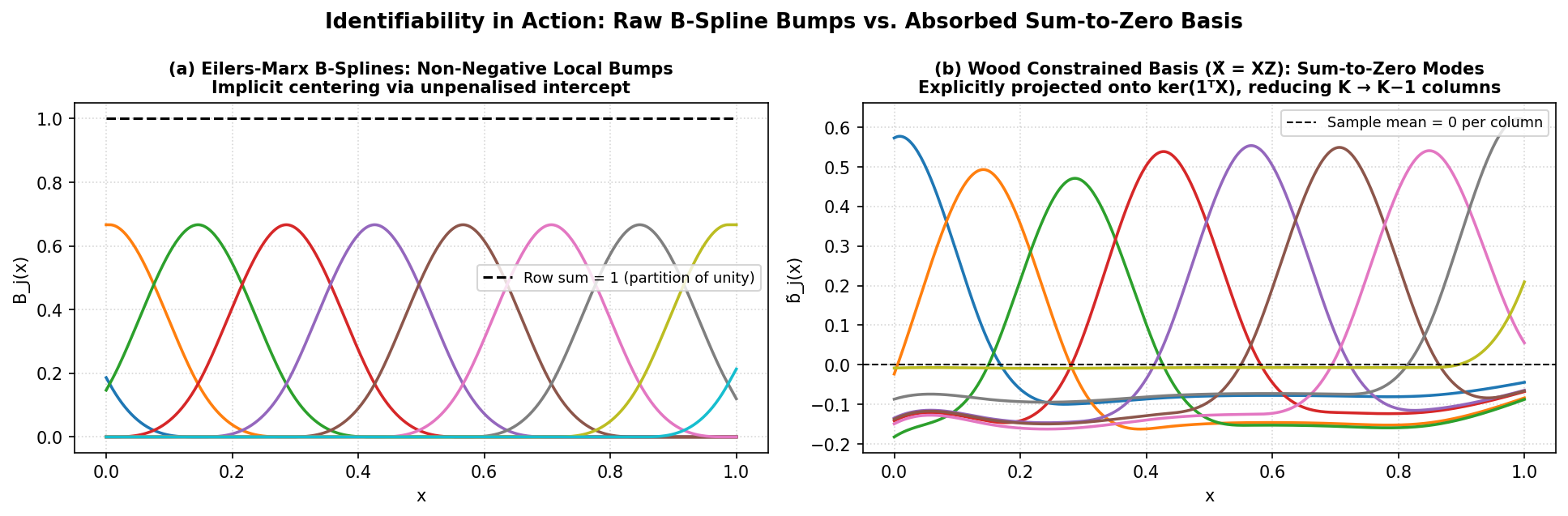
Comparison of uncentred Eilers-Marx B-spline bumps versus Wood sum-to-zero projected basis functions — The left panel shows that Eilers-Marx B-spline basis columns ($K = 8$) are non-negative and satisfy the partition of unity $\sum_j B_j(x) = 1$, meaning any constant shift can be traded with the intercept. The right panel shows how Wood’s `absorb_constraints` projects the basis onto the $(K-1)$-dimensional subspace where every column has zero sample mean ($\mathbf{1}^\top \tilde{X} = \mathbf{0}$), guaranteeing a unique, zero-centred partial effect.¶

For tensor-product terms the same pipeline applies after assembling the Kronecker-sum penalties; each marginal penalty is first normalised by its largest eigenvalue (so the dimensions contribute to the penalty on equal footing), then the usual S.scale + absorb.cons pass runs on the full tensor basis.

Smoothing Parameter Selection with REML and GCV.Cp¶

Both backends minimise the same penalised objective,

\[\| \mathbf{y} - X\boldsymbol{\beta} \|^2 + \sum_i \lambda_i \boldsymbol{\beta}^\top S_i \boldsymbol{\beta} = \| \mathbf{y} - X\boldsymbol{\beta} \|^2 + \boldsymbol{\beta}^\top S_{\boldsymbol{\lambda}} \boldsymbol{\beta},\]

but they choose $\boldsymbol{\lambda}$ differently. The Eilers-Marx backend sweeps a grid and scores each point with GCV. The Wood backend treats $\boldsymbol{\lambda}$ as continuous parameters of a model-selection criterion and optimises. For a fixed $\boldsymbol{\lambda}$, the fit is obtained by QR of $X$ and a Cholesky solve of

\[H = R^\top R + S_{\boldsymbol{\lambda}} = L L^\top, \qquad \hat{\boldsymbol{\beta}} = H^{-1} X^\top \mathbf{y}.\]

(With the tiny ridge on $H$’s diagonal guarding the $\lambda = 0$ edge case.)

GCV.Cp. The same criterion as the Eilers-Marx backend, computed from the Cholesky factor instead of an SVD. The EDF is

\[\text{EDF} = \operatorname{tr}(H^{-1} R^\top R) = \| L^{-1} R^\top \|_F^2,\]

(using the trace identity $\operatorname{tr}(ABA^\top) = \|AB^{1/2}\|_F^2$ with $A = R$, $B = H^{-1} = L^{-\top}L^{-1}$), and the score is

\[V_g(\boldsymbol{\lambda}) = \frac{n \cdot \text{RSS}}{(n - \gamma \cdot \text{EDF})^2}, \qquad \hat\sigma^2 = \frac{\text{RSS}}{n - \text{EDF}}.\]

Here the default $\gamma = 1$ (GCV.Cp), versus 1.4 in the Eilers-Marx backend, a small but real difference between the two engines’ model-selection tastes.

REML (the default). Give the coefficients a Gaussian prior whose precision is the penalty,

\[\mathbf{y} = X\boldsymbol{\beta} + \boldsymbol{\varepsilon}, \quad \boldsymbol{\varepsilon} \sim N(0, \sigma^2 I), \qquad \boldsymbol{\beta} \sim N\bigl(0, \,\sigma^2 S_{\boldsymbol{\lambda}}^{-}\bigr),\]

where $S_{\boldsymbol{\lambda}}^{-}$ denotes the (generalised) inverse, representing an improper prior that treats the penalty’s null space as infinite variance. Integrating $\boldsymbol{\beta}$ out gives the marginal (restricted) likelihood for $\boldsymbol{\lambda}$ and $\sigma^2$. Profiling out $\sigma^2$ at

\[\hat\sigma^2 = \frac{D_p}{n - M_p}, \qquad D_p = \underbrace{\|\mathbf{y} - X\hat{\boldsymbol{\beta}}\|^2}_{\text{RSS}} + \underbrace{\hat{\boldsymbol{\beta}}^\top S_{\boldsymbol{\lambda}} \hat{\boldsymbol{\beta}}}_{\text{penalty cost}},\]

where $M_p = p - \operatorname{rank}(S_{\boldsymbol{\lambda}})$ is the total unpenalised null-space dimension of the model (the intercept plus any unpenalised polynomial modes in the smooths), the criterion to minimise is

\[\ell_r(\boldsymbol{\lambda}) \;=\; \frac{D_p}{2\hat\sigma^2} + \frac{n - M_p}{2} \log(2\pi\hat\sigma^2) + \frac12 \log |H| - \frac12 \log |S_{\boldsymbol{\lambda}}|_+ .\]

Each component in this score has an intuitive interpretation:

The first term, $D_p / (2\hat\sigma^2)$, measures goodness of fit by evaluating how closely the penalized curve tracks the observations relative to the estimated residual noise.
The second term, $\frac12 \log|H|$, acts as an explicit complexity penalty. When you weaken the smoothing penalty, the determinant of $H$ swells, penalizing over-flexible models and preventing $\lambda \to 0$.
The third term, $-\frac12 \log|S_{\boldsymbol{\lambda}}|_+$ provides the normalization constant for the Gaussian prior. Because the penalty matrix has a null space for flat or linear functions, this determinant is evaluated over positive eigenvalues only (:math:`|S|_+$), avoiding the undefined logarithm of zero while correctly adjusting for the rank of the penalty.

Why the positive-eigenvalue determinant matters can be seen by taking $S_\lambda = \lambda S$ with $\operatorname{rank}(S) = r$, yielding $\log|S_\lambda|_+ = r\log\lambda + \log|S|_+$, which scales correctly with the rank. When each penalty acts on its own disjoint block of coefficients, _precompute_penalty_structure precomputes the rank and positive eigenvalues once:

\[\log |S_{\boldsymbol{\lambda}}|_+ = \sum_i \Bigl[ \operatorname{rank}(S_i) \log \lambda_i + \sum_j \log \text{ev}^+_j(S_i) \Bigr],\]

When multiple penalties overlap on the same coefficient block (such as the marginal penalties of a te() tensor smooth), the implementation projects each component onto the positive eigenspace of $\sum_i S_i$ once, and evaluates $\log |S_{\boldsymbol{\lambda}}|_+$ via a pre-balanced Cholesky factorisation of the reduced positive-definite matrix (falling back to eigvalsh only if needed).

$\log|H|$ needs no eigendecomposition: from the Cholesky factor, $\log|H| = 2\sum_i \log L_{ii}$.

Why REML and not maximum likelihood? In the mixed-model view, estimating $\boldsymbol{\beta}$ costs degrees of freedom; plain ML ignores this and biases $\sigma^2$ (and thus $\lambda$) downward and under-smoothes. The restricted likelihood corrects for exactly this loss, which is why the criterion uses $n - M_p$ instead of $n$. REML also has better-behaved optima than GCV, which is notorious for flat minima and occasional near-zero $\lambda$ solutions.

Optimising in log space. $\lambda$ must be positive, so the backend optimises $\rho = \log\lambda$ (unconstrained, with $\lambda = e^\rho$) over the range $\rho \in [-15, 15]$: i.e. $\lambda$ between roughly $3\times10^{-7}$ and $3\times10^{6}$. Both single- and multi-penalty models use L-BFGS-B with exact analytic gradients (jac=True), seeded from the best point on a coarse initial grid $\rho_0 \in \{-8, -4, 0, 4, 8\}$ to avoid flat-tail trapping. Because the envelope theorem cancels the implicit $\partial\hat{\boldsymbol{\beta}}/\partial\rho_j$ terms in $\partial D_p / \partial\rho_j = \lambda_j \hat{\boldsymbol{\beta}}^\top S_j \hat{\boldsymbol{\beta}}$, both the REML and GCV gradients fall out of the existing Cholesky factor $L$ in a single pass without finite-difference evaluations. Individual $\lambda$ values can be pinned with sp= if you want some terms fixed and others estimated, and model.gridsearch() is also available on Wood models if you wish to search over candidate basis dimensions $k$ while REML/GCV optimises $\boldsymbol{\lambda}$ continuously at each candidate $k$.

The REML score itself is reported in statistics_ along with the estimated $\lambda$ values, so you can compare models on the restricted likelihood.

Inference with Two Covariances and Wood’s F-Test¶

With $\boldsymbol{\lambda}$ estimated, the backend computes a full inferential kit. Two covariance matrices appear:

\[V_p = H^{-1}\hat\sigma^2, \qquad V_e = H^{-1} X^\top X H^{-1} \hat\sigma^2 = H^{-1} R^\top R H^{-1} \hat\sigma^2.\]

$V_p$ is the Bayesian posterior covariance, representing the posterior of $\boldsymbol{\beta}$ under the prior that generated REML, with $\lambda$ treated as known. It is what the Wood backend reports in summary() tables and uses for confidence bands; standard errors are $\operatorname{SE}_j = \sqrt{(V_p)_{jj}}$.
$V_e$ is the frequentist (sandwich) covariance, representing the sampling covariance of $\hat{\boldsymbol{\beta}}$ treating the penalty as part of the estimator, again with $\lambda$ fixed. It ignores the uncertainty in $\lambda$ itself (a standard simplification in Wood’s formulation, though the literature notes it makes intervals slightly optimistic).

Interval widths for a new point $\mathbf{x}^*$ come from $\mathbf{x}^{*\top} V_p \,\mathbf{x}^*$, with $\hat\sigma^2$ added for prediction intervals; the implementation uses t quantiles with $n - \text{EDF}$ degrees of freedom.

Per-coefficient and per-term EDF. From the influence matrix

\[F = H^{-1} R^\top R, \qquad \text{EDF} = \operatorname{tr}(F), \qquad \text{EDF}_j = F_{jj}.\]

Term-level EDF is the sum of $F_{jj}$ over that term’s coefficient block. A term with EDF near 1 is essentially linear; a term whose EDF barely exceeds 1 despite a large $k$ is doing very little.

Wood’s approximate F-tests. For each term, testing $H_0:\; f_j = 0$ (in basis terms, $\boldsymbol{\beta}_j = 0$), the Wood backend uses the test statistic (Wood 2013)

\[F_j = \frac{\hat{\boldsymbol{\beta}}_j^\top V_{p,j}^{-1} \hat{\boldsymbol{\beta}}_j} {\text{EDF}_j} \;\sim\; F(\text{EDF}_j,\; n - \text{EDF}_{\text{total}}) \;\; \text{under } H_0,\]

with the p-value from the right tail of the F distribution. The justification relies on a moment-matching argument where under the null the quadratic form has mean $\text{EDF}_j$ and variance $2\,\text{EDF}_j$, matching an $F$-like distribution to second order. It is an approximation, exact for $\lambda = 0$ (where it reduces to the classical F-test) and well-calibrated for EDF comfortably above 1, but p-values for terms with EDF barely above 1 should be read with suspicion (a known caveat in Wood 2013).

Model-level summaries. The backend also reports:

\[\text{deviance explained} = 1 - \frac{\text{RSS}}{\sum_i (y_i-\bar y)^2}, \qquad R^2_{\text{adj}} = 1 - \frac{\text{RSS}/(n-\text{EDF})} {\text{TSS}/(n-1)},\]

the Gaussian log-likelihood $\ell = -\tfrac{n}{2}\log(2\pi\hat\sigma^2) - \tfrac{\text{RSS}}{2\hat\sigma^2}$, and the information criteria $\text{AIC} = -2\ell + 2(\text{EDF}+1)$, $\text{BIC} = -2\ell + \log(n)(\text{EDF}+1)$, with $+1$ counting the estimated $\sigma^2$. These make the Wood backend the choice when you need p-values, AIC-based model comparison, or output that matches an R summary.gam table.