Shape Constraints

magli supports shape constraints on univariate spline terms (s()) and on GAM / LinGAM. In backend='eilers', monotonicity and convexity constraints are enforced via pyGAM’s iterative active-set asymmetric difference penalty on violated B-spline coefficient differences, while periodicity wraps the B-spline basis and penalty across the domain boundaries.

Note

Monotonicity and convexity constraints (mono_inc, mono_dec, convex, concave) are provided by the Eilers-Marx engine (backend='eilers'). Periodic smooths (constraint='periodic') are supported in both engines, using wrapped B-splines in backend='eilers' and via cyclic cubic/P-spline bases (bs='cc' / bs='cp') in backend='wood'.

Available constraints

Constraint	Penalty	Effect
None	\(\lambda D_2^\top D_2\)	Standard smoothness (default)
mono_inc	\(\lambda D_2^\top D_2 + C_{\text{inc}}(\beta)\)	Enforces monotonically increasing curve (\(\Delta\beta_j \ge 0\))
mono_dec	\(\lambda D_2^\top D_2 + C_{\text{dec}}(\beta)\)	Enforces monotonically decreasing curve (\(\Delta\beta_j \le 0\))
convex	\(\lambda D_2^\top D_2 + C_{\text{cvx}}(\beta)\)	Enforces convexity (U-shaped, \(\Delta^2\beta_j \ge 0\))
concave	\(\lambda D_2^\top D_2 + C_{\text{ccv}}(\beta)\)	Enforces concavity (∩-shaped, \(\Delta^2\beta_j \le 0\))
periodic	Circular \(\lambda D_2^\top D_2\) / cyclic	Enforces \(f(a) = f(b)\) with wrapped basis and penalty (both backends)

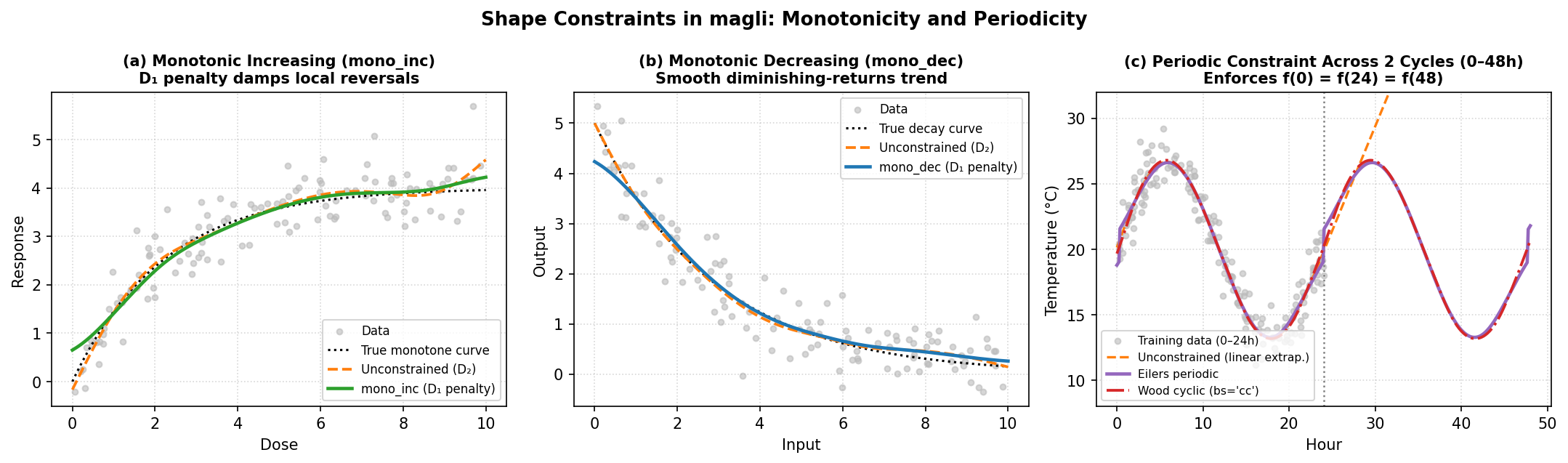
Effect of shape constraints on noisy data, where (left) constraint='mono_inc' suppresses non-physical local dips in a dose-response curve; (centre) constraint='mono_dec' damps rebounds in an exponential decay curve; (right) constraint='periodic' (or Wood’s bs='cc') joins value and slope seamlessly across the 24-hour cycle boundary.

How they work

Monotonicity and convexity combine the standard smoothness penalty \(\lambda D_2^\top D_2\) with an iterative active-set penalty \(C(\boldsymbol{\beta})\):

\[C(\boldsymbol{\beta}) = \lambda_{\text{con}} \, D_m^\top \operatorname{diag}\bigl(\mathbf{v}(\boldsymbol{\beta})\bigr) D_m + \lambda_{L2} I,\]

where \(\lambda_{\text{con}} = 10^9\), \(\lambda_{L2} = 10^{-3}\), and \(\mathbf{v}(\boldsymbol{\beta}) \in \{0, 1\}^{K-m}\) indicates which first differences (\(m=1\) for mono_inc / mono_dec) or second differences (\(m=2\) for convex / concave) violate the target sign:

• mono_inc penalises \(\Delta\beta_j = \beta_{j+1} - \beta_j < 0\).

• mono_dec penalises \(\Delta\beta_j = \beta_{j+1} - \beta_j > 0\).

• convex penalises \(\Delta^2\beta_j = \beta_{j+2} - 2\beta_{j+1} + \beta_j < 0\).

• concave penalises \(\Delta^2\beta_j = \beta_{j+2} - 2\beta_{j+1} + \beta_j > 0\).

Because the variation-diminishing property of B-splines guarantees that a B-spline with monotone (or convex/concave) coefficients is itself monotone (or convex/concave), iteratively updating \(\mathbf{v}(\boldsymbol{\beta})\) until convergence produces a smooth curve satisfying the directional shape constraint.

Periodicity wraps the basis and penalty:

• The B-spline basis is evaluated on \([0,1]\) with \(z = z \bmod 1\), so the domain is a circle.

• The last \(k\) columns are folded into the first \(k\) columns, preserving the partition of unity \(\sum_j B_j(x) = 1\) and reducing the coefficient count from \(K\) to \(K_{\text{eff}} = K - k\).

• The circular second-difference penalty connects index \(K_{\text{eff}}\) back to index 1 with \(C^2\) continuity across the boundary.

When to use which

• Monotonic increasing: dose-response curves, learning curves, cumulative distributions, prices vs. demand.

• Monotonic decreasing: diminishing returns, survival curves, price elasticity.

• Convex: cost functions, loss landscapes, risk curves.

• Concave: utility functions, production functions.

• Periodic: time-of-day effects, seasonal patterns, angular coordinates (compass directions).

Caveats

1. Sufficient condition via B-spline coefficients. Enforcing \(\Delta^2\beta_j \ge 0\) on B-spline control points is a sufficient (slightly conservative) condition for convexity of \(f(x)\).

2. Intercept is free. The intercept column is never penalised, so the overall vertical shift is unrestricted.

3. Periodicity reduces capacity. A periodic spline with \(K=10\) and \(k=3\) has \(K_{\text{eff}} = K - k = 7\) free coefficients. You may need slightly larger n_splines to capture the same complexity as a non-periodic spline.

4. Not available for ``te()``. Tensor-product terms do not support shape constraints because the multi-dimensional penalty structure does not admit a simple ordered-difference formulation. Apply constraints to the marginal s() terms instead.

Examples

Monotonically increasing spline:

model = GAMCore("s(0, constraint='mono_inc') + l(1)", backend="eilers")
model.fit(x, y)

Periodic seasonal effect:

model = GAMCore("s(0, n_splines=12, constraint='periodic') + l(1)", backend="eilers")
model.fit(x, y)

Single-term with monotonicity:

model = LinGAM(n_splines=12, constraint='mono_inc', backend="eilers")
model.fit(x, y)